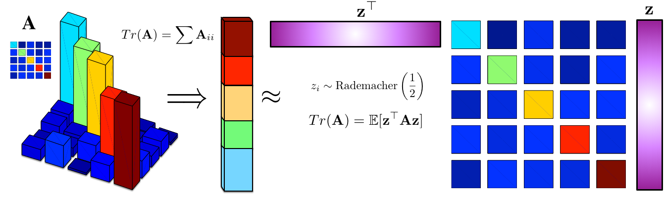
Hutchinson's estimator [cite key='hutchinson1990stochastic'] is a simple way to obtain a stochastic estimate of the trace of a matrix. This is a simple trick that uses randomisation to transform the algebraic problem of computing the trace into the statistical problem of computing an expectation of a quadratic function. The randomisation technique used in this trick is just one from a wide range of randomised linear algebra methods [cite key='mahoney2011randomized'] that are now central to modern machine learning, since they provide us with the needed tools for general-purpose, large-scale modelling and prediction. This post examines Hutchinson's estimator and the wider research area of randomised algorithms.

Stochastic Trace Estimators

We are interested in a general method for computing the trace of a matrix with a randomised algorithm. Hutchinson's and other closely related estimators [cite key='hutchinson1990stochastic'] do this using a simple identity:

   

z is a random variable that is typically Gaussian or Rademacher distributed. We obtain a randomised algorithm by solving the expectation by Monte Carlo using draws of z from its distribution, evaluating the quadratic term, and averaging. This exposes an interesting duality between the trace and expectation operators.

Consider a multivariate random variable z with mean

   

and variance

   

. Using the property of expectations of quadratic forms, the expectation

   

. Furthermore, for zero-mean, unit-variance random variables, this implies that

   

, which is what will enable our randomised algorithm. We can now easily derive this class of trace estimators ourselves:

   

   

If you sample z from a Rademacher distribution, whose entries are either -1 or 1 with probability 0.5, then this estimator is known as Hutchinson's estimator.  But we can also use a Gaussian or other distribution — our main requirement is the ability to sample easily from our chosen distribution.

Estimator variance

We have derived an unbiased estimator of the trace, and the usual next question that is asked is what we can say about its variance (low variance will give us more confidence in its use). We can compare the variance for the most commonly used random variables: the Rademacher and the Gaussian.

To derive the variance for the Rademacher distribution, we will need to exploit many of its properties. In particular, it has zero mean and unit variance. It is also a symmetric distribution, which implies that all its odd central moments are zero. Its 2nd central moment (variance)

   

and its excess kurtosis is -2, which implies that its 4th central moment

   

. All this is needed for us to use the expression for the variance of general quadratic forms [§5.1.2][cite key='petersen2008matrix']. Let

   

.

   

The 2nd and 3rd terms are zero because the mean m is zero. This simplifies the expression to:

   

   

For Gaussian distributed z, the variance is easier (

   

) and is: 

   

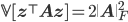
The variance using the Rademacher distribution (Hutchinson's estimator) has lower variance compared to the Gaussian, and is one reason it is often preferred. We can also compute a bound on the number of samples needed by the Monte Carlo estimator to obtain an error of at most

   

with probability

   

[cite key='avron2011randomized']:

• Rademacher:

     

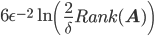
• Gaussian: 

     

The story is different now and the Gaussian requires fewer samples. But these bounds are not tight, and many practitioners have found there to be little difference between the Gaussian and Rademacher cases.

Randomised Algorithms

Hutchinson's estimator shows one way in which randomisation and Monte Carlo can be used to reduce the computational complexity of common linear algebra operations. Hutchinson's estimator is widely used since trace terms are ubiquitous. Trace terms appear:

• When computing the KL divergence between two Gaussian distributions;
• When we compute derivatives of log-determinants, norms and many structured matrices, e.g., in the gradient of the marginal likelihood of Gaussian process models;
• When computing expectations and higher-order moments of polynomials of random variables.

As a concrete example*, a common problem that must be solved when optimising the marginal likelihood in Gaussian processes, is to compute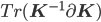

   

. A direct computation has cubic complexity due to the inversion and matrix multiplication. We can reduce this complexity by using Hutchinson's estimator:

   

   

Computing an unbiased estimator of our initial trace problem can now be computed using only systems of linear equations, which is computationally cheaper than the direct method. One recent paper where this has been used for scalable probabilistic inference is [cite key='filippone2015enabling']:

• Enabling scalable stochastic gradient-based inference for Gaussian processes by employing the Unbiased LInear System SolvEr (ULISSE).

The tool of randomisation that is exploited by Hutchinson's estimator is very powerful and can be used in many ingenious ways:

• Michael Mahoney [cite key='mahoney2011randomized'] provides some essential reading that covers the basics of randomised linear algebra, showing how we can solve least squares and matrix factorisation problems.
  • Randomized algorithms for matrices and data.
• The QR decomposition and SVD are core components of many machine learning algorithms, and there is much work that shows us how to scale-up these algorithms using randomised approximations.
  • Finding structure with randomness: Probabilistic algorithms for constructing approximate matrix decompositions.
• The celebrated Johnson-Lindenstrauß lemma (or flattening lemma) is widely known, and allows us to do randomised dimensionality reduction.
  • This can then be exploited in many interesting ways, such as in compressed sensing or for scaling Bayesian optimisation.
• Randomised algorithms can be used for scalability across the machine learning pipeline. This is where randomised algorithms such as sketching, hashing and approximate nearest neighbours come into play. The book by Mitzenmacher and Upfal [cite key=mitzenmacher2005probability] is one very good introduction to this area.

Summary

Hutchinson's estimator allows us to compute a stochastic, unbiased estimator of the trace of a matrix. It forms one instance of a diverse set of randomised algorithms for matrix algebra that we can use to scale up our machine learning systems. A large class of modern machine learning requires such tools to handle the size of data we are now routinely faced with, making these randomised algorithms amongst our most welcome of tricks.

[*Thanks to Maurizio Filippone for introducing me to this trick.]

[bibsource file=http://www.shakirm.com/blog-bib/trickOfTheDay/hutchinsonsTrick.bib]