· Read in 8 minutes · 1499 words · All posts in series ·
[dropcap]This[/dropcap] trick is unlike the others we've conjured. It will not reveal a clever manipulation of a probability or an integral or a derivative, or produce a code one-liner. But like all our other tricks, it will give us a powerful instrument in our toolbox. The instruments of thinking are rare and always sought-after, because with them we can actively and confidently challenge the assumptions and limitations of our machine learning practice. Something we must constantly do.
One of the most common tasks we can attempt with data is to use features x to make predictions of targets y. This regression often makes a key assumption: any noise ![\[\epsilon\]](http://blog.shakirm.com/wp-content/ql-cache/quicklatex.com-d7b18f78571c458e567622238f3c07ae_l3.png "Rendered by QuickLaTeX.com")
![\[\mathbf{y}_n = \boldsymbol{\beta}^\top\mathbf{x}_n +\boldsymbol{\epsilon}\]](http://blog.shakirm.com/wp-content/ql-cache/quicklatex.com-63e8f92e75a04140be69fc5b9d021870_l3.png "Rendered by QuickLaTeX.com")
If this assumption is actually true for the problem we are addressing—that features x are linearly related to targets y using a set of parameters ![\[\beta\]](http://blog.shakirm.com/wp-content/ql-cache/quicklatex.com-9dd9202d5c8ce4000957f0b13db4c135_l3.png "Rendered by QuickLaTeX.com")

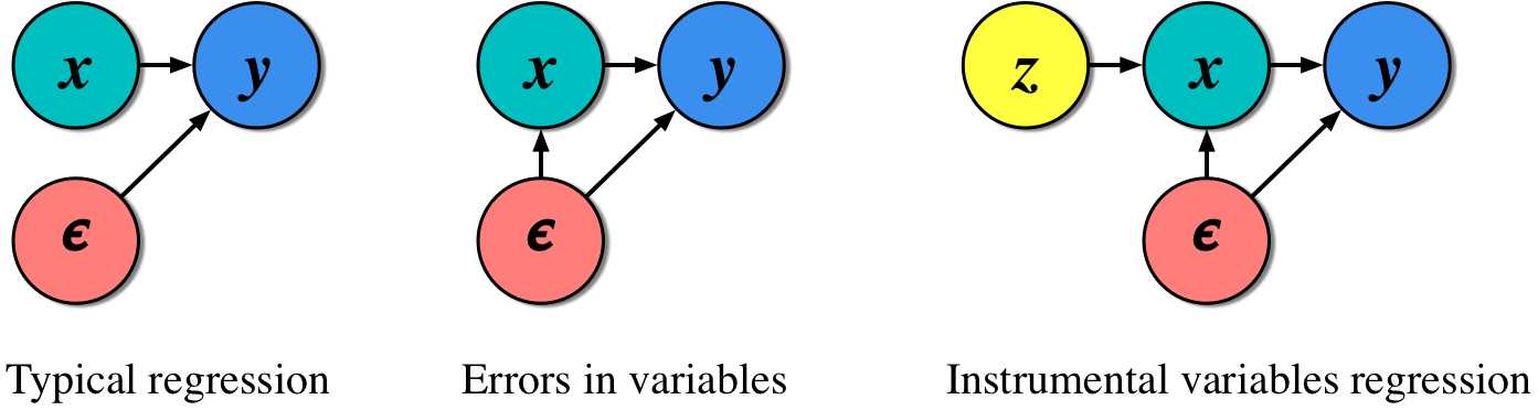
Figure 1. Three common regression scenarios.
Learning with Errors in Variables
Consider what is known as an errors-in-variables scenario1 (see figure 1 (centre)): a regression problem where the same source of noise
If we ever find ourselves in this situation, then we no longer have a structural equation; any model we have will simply track correlations in the data and will leave us with biased predictions. This is where our trick of the day enters. The instrumental variables trick asks us to use the data itself to account for noise, and makes it easier for us to define structural models and to make causal predictions.
The instrumental variables idea is conceptually simple: we introduce new observed variables z, called instrumental variables, into our model; figure 1 (right). And this is the trick: instrumental variables are special subset of the data we already have, but they allow us to remove the effect of confounders. Confounders are the noise and other interactions in our system whose effect we may not know or be able to observe, but which affect our ability to write structural models. We manipulate these instruments so that we transform the undesirable regression in figure 1(centre) into a structural regression of the form of figure 1 (left).
For a variable to be an instrumental variable, it must satisfy two conditions:
- The instruments z should be (strongly) correlated with the features x. There should be a direct association between the instrument and the data we wish to use to make predictions.
- The instruments should be uncorrelated with the noise
. This says that changes in instruments z should lead to changes in x, but not to y; otherwise z would be subject to the same errors-in-variables problem.
The common example is the prediction of future earnings (y) based on education (x). A person's ability (
Two-stage Least Squares
The instrumental variables construction simply says that we should remove (marginalise) the effect of the variables (x) that have coupled errors, and instead consider the following marginalised distribution:
![\[p(\mathbf{y} | \mathbf{z}) = \int p_\theta(\mathbf{y} |\mathbf{x}) p_\phi(\mathbf{x} |\mathbf{z}) dx\]](http://blog.shakirm.com/wp-content/ql-cache/quicklatex.com-4484395d045253b5f960c37a4fdd5b61_l3.png "Rendered by QuickLaTeX.com")
Where ![\[\theta\]](http://blog.shakirm.com/wp-content/ql-cache/quicklatex.com-4c29edd802429cf80b07b851f997cf63_l3.png "Rendered by QuickLaTeX.com")
![\[\phi\]](http://blog.shakirm.com/wp-content/ql-cache/quicklatex.com-56d9aee3b38ebdbfb319fbb130f7baa0_l3.png "Rendered by QuickLaTeX.com")
- Train a model to predict the inputs x given instruments z. This can be a regression model, or a more complex high-dimensional conditional generative model. Call these predictions
.![\[\hat{\mathbf{x}}\]](http://blog.shakirm.com/wp-content/ql-cache/quicklatex.com-0087471cfb5de1dfe9d0657a9abde605_l3.png "Rendered by QuickLaTeX.com")
- We now train a model to predict targets y given the predicted inputs
.
If a linear regression model is used for both these steps, then we will recover the famous two-stage least squares (2SLS) algorithm. Using the closed form solution (the normal equations) for each stage of the regression, we get:
Stage 1: Feature prediction using instruments
- Optimal parameters:
![\[\boldsymbol{\phi} = (\mathbf{Z}^\top\mathbf{Z})^{-1}\mathbf{Z}^\top \mathbf{X}\]](http://blog.shakirm.com/wp-content/ql-cache/quicklatex.com-104746ee5a71d4a24f9d09bd0384f65d_l3.png "Rendered by QuickLaTeX.com")
- Predictions:
![\[\hat{\mathbf{X}}=\mathbf{Z}\mathbf{\phi}=\mathbf{Z}(\mathbf{Z}^\top\mathbf{Z})^{-1}\mathbf{Z}^\top \mathbf{X} =\mathbf{P}_z\mathbf{X}\]](http://blog.shakirm.com/wp-content/ql-cache/quicklatex.com-8aa89b415f037fb9485a6cb60ba664d8_l3.png "Rendered by QuickLaTeX.com")
Stage 2: Target prediction using predicted features
- Optimal stage 2 parameters:
![\[\boldsymbol{\theta} = (\hat{\mathbf{X}}^\top\hat{\mathbf{X}})^{-1}\hat{\mathbf{X}}^\top \mathbf{y} = (\mathbf{X}\mathbf{P}_z\mathbf{X})^{-1}\mathbf{X}^\top\mathbf{P}_z\mathbf{y}\]](http://blog.shakirm.com/wp-content/ql-cache/quicklatex.com-5a7d4e8cc5f5fec53f7042af8d49f70e_l3.png "Rendered by QuickLaTeX.com")
2SLS does something intuitive: by introducing the instrumental variable, it creates a way to eliminate the paths through which confounding noise enters the model to create an errors-in-variables scenario. Using the predicted inputs ![\[\hat{x}\]](http://blog.shakirm.com/wp-content/ql-cache/quicklatex.com-51e5fae837ff4df71995aec3f75d7c0a_l3.png "Rendered by QuickLaTeX.com")
There are many powerful real-word examples where this thinking has been used, especially in settings where we cannot do randomised control trials but must rely on observational data. There is much more that could be written about these applications alone. Yet, how often will we have a situation in which we have an additional source of data to use as an instrument?
Instrumental variables are hard to find in real-world problems. And the assumption, hidden in the use of the Normal equations, that the number of instruments we use is the same as the number of input features (called the just-specified case), makes it difficult in high-dimensional problems. But the power of instrumental variables is not lost. They still shine, especially in settings where we control the definition of all the variables involved. One such area is reinforcement learning.
Reinforcement Learning with Instruments
It may not look like it, but the problem of learning value-functions is an errors-in-variables scenario. Our problem is to learn a linear value function using features ![\[s_x\]](http://blog.shakirm.com/wp-content/ql-cache/quicklatex.com-227f3454074f3b49475674b56ea765ff_l3.png "Rendered by QuickLaTeX.com")
![\[V(x) = s_x^\top\theta\]](http://blog.shakirm.com/wp-content/ql-cache/quicklatex.com-0f1a2436d37ed070287b699380d15bec_l3.png "Rendered by QuickLaTeX.com")
Let's start from the definition of the value function under transition distribution ![\[p(x,x')\]](http://blog.shakirm.com/wp-content/ql-cache/quicklatex.com-b6d90f36bd287dbea5dd998f79ee713b_l3.png "Rendered by QuickLaTeX.com")
![\[R(x,x')\]](http://blog.shakirm.com/wp-content/ql-cache/quicklatex.com-a2d76022df0b0a0c5708ac6e9de50880_l3.png "Rendered by QuickLaTeX.com")
![\[\gamma\]](http://blog.shakirm.com/wp-content/ql-cache/quicklatex.com-24edd3bc089c270b2a78b63b8ac9f5de_l3.png "Rendered by QuickLaTeX.com")
![\[V(x) = \sum_{x'}p(x,x')[R(x,x') + \gamma V(x')] = \bar{r}_x +\gamma \sum_{x'}p(x,x')V(x').\]](http://blog.shakirm.com/wp-content/ql-cache/quicklatex.com-9df13dd7f8ad8cf853fcbe6a06e02167_l3.png "Rendered by QuickLaTeX.com")
We can also rewrite the value function as an expected immediate reward ![\[\bar{r}_x =\sum_{x'}p(x,x')R(x,x')\]](http://blog.shakirm.com/wp-content/ql-cache/quicklatex.com-ad0fad2bf9586023957e3f16c91995b4_l3.png "Rendered by QuickLaTeX.com")
![\[\bar{r}\]](http://blog.shakirm.com/wp-content/ql-cache/quicklatex.com-ca3d421379c5cdd46a6f966ca4f000b6_l3.png "Rendered by QuickLaTeX.com")
![\[\bar{r}_x = s_x^\top\theta - \gamma\sum_{x'}p(x,x')s_{x'}^\top\theta) = (\underbrace{s_x -\gamma\sum_{x'}p(x,x')s_{x'}}_{\Delta})^\top\theta.\]](http://blog.shakirm.com/wp-content/ql-cache/quicklatex.com-a6d7440cf04e06604d913fa64b1c99f1_l3.png "Rendered by QuickLaTeX.com")
This is a regression from features that capture the change-in-state ![\[\Delta\]](http://blog.shakirm.com/wp-content/ql-cache/quicklatex.com-cabd1bc6f3aa1205cb73e077a64e5933_l3.png "Rendered by QuickLaTeX.com")
![\[\bar{r}_x\]](http://blog.shakirm.com/wp-content/ql-cache/quicklatex.com-6b4b2ffac5de8d52791b577ac1d65693_l3.png "Rendered by QuickLaTeX.com")
But we do have a trick for such scenarios: we can use instrumental variables regression and remain able to learn value-function parameters that correctly capture the causal structure of future rewards.
Because we control this setting, with a bit of thought, we can conclude that a set of instrumental variables that are strongly correlated with the features ![\[s\]](http://blog.shakirm.com/wp-content/ql-cache/quicklatex.com-18e24c008672f52d5c119fb3f3eef234_l3.png "Rendered by QuickLaTeX.com")
Stage 1: Instrumental variables regression
- Linear instrumental parameters:
![\[\phi = (S_t^\top S_t)^{-1}S_t^\top\Delta\]](http://blog.shakirm.com/wp-content/ql-cache/quicklatex.com-0ef2b258c94ea233570b125631e4941a_l3.png "Rendered by QuickLaTeX.com")
- Instrumental prediction:
![\[\hat{\Delta}=S_t^\top\phi\]](http://blog.shakirm.com/wp-content/ql-cache/quicklatex.com-03cfa27cacade4c6444d0c1eccddaa52_l3.png "Rendered by QuickLaTeX.com")
Stage 2: Average reward prediction
- Parameter estimation:
![\[\theta = (S_t^\top\Delta)^{-1}S_t^\top r_t\]](http://blog.shakirm.com/wp-content/ql-cache/quicklatex.com-73d379e93bce05ddfb2cfdbcb433e276_l3.png "Rendered by QuickLaTeX.com")
In reinforcement learning, this approach is known as Least squares TD (LSTD) learning. Most RL will instead reach this conclusion using the theory of Bellman projections. But this probabilistic viewpoint through instrumental variables means that we can think of alternative ways of extending this view.
We can go much deeper, and these papers can be used to explore this topic further:
- Tutorial in Biostatistics: Instrumental Variable Methods for Causal Inference
- Linear Least-Squares algorithms for temporal difference learning
- LASSO Methods for Gaussian Instrumental Variables Models
- Learning Instrumental Variables with Structural and Non-Gaussianity Assumptions
- Deep Instrumental Variables: A Flexible Approach for Counterfactual Prediction
Summary
The instrumental variables tell us to critically consider the assumptions underlying the models we develop and to think deeply about how to use their predictions correctly. The importance of this for our machine learning practice cannot be overstated.
Like every trick in this series, the instrumental variables give us an alternative way to think about existing problems. It is to find these alternative views that I write this series, and is the real reason to study these tricks at all: they give us new ways to see.
Complement this trick with other tricks in the series. Or read one my earliest pieces on a Widely-applicable information criterion, or a piece of exploratory thinking on Decolonising artificial intelligence.
Im a little confused and hope you could expand on a couple things:
1) The definition of an instrumental variable doesn't seem very clear to me. If you have variables which can predict y (in your example it was personal ability) that variable should be in the x block. It isn't an error estimator, it's a direct correlate to the y variable. I'm also unsure how it adds error to your x variable, as education and ability are different direct measurables.
In short, I don't see how this changes the simple linear regression equation. You may have variables with higher impact on y, certainly. You may also have noise in your measurements (e.g. white noise in a spectral dataset). Yet your description claws at something greater and I'm having a hard time seeing it.
2) is this math significantly different than a PCA or PLS calculation? You've pre-selected your z-variables (it seems) and then computed a y variable from this limited selection. I can't recall the math directly bur it seems quite similar.