The NIPS 2014 Workshop on Advances in Variational Inference was abuzz with new methods and ideas for scalable approximate inference. The concluding event of the workshop was a lively debate with David Blei, Neil Lawrence, Zoubin Ghahramani, Shinichi Nakajima and Matthias Seeger on the history, trends and open questions in variational inference. One of the questions posed to our panel and audience was: 'what are your variational inference tricks-of-the-trade?'
My current best-practice at present includes: stochastic approximation, Monte Carlo estimation, amortised inference and powerful software tools. But this is a though-provoking question that has has motivated me think in some more detail through my current variational inference tricks-of-the-trade, which are:
Stochastic approximation as a default
The ability to use our models in the mini-batch setting has become an essential tool to allow us to perform probabilistic reasoning over large data sets. As a results, gradient-based updates using stochastic gradient ascent, and hence stochastic variational inference, is now one of the must-have tools in our box of tricks [cite key="hoffman2012stochastic"].
Recognition models and amortised inference

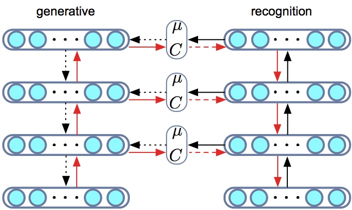
A recognition model or inference network is a model that learns an inverse map from observations to latent variables. This is a mechanism with which we can share statistical strength and generalisation between the inferences made for each observation and amortise the cost of inference. By using a recognition model, every inference computation contributes to better inference for all other data points (and unseen data points) and can allow for faster convergence during training and faster inference at test time [cite key="stuhlmuller2013learning"][cite key="gershman2014"][cite key="rezende2014"].
The use of recognition models also connects variational inference in directed graphical models to other other encoder-decoder systems such as compression models and auto-encoders. Using variational inference we have the benefit that we begin with a known probabilistic description of our data (the generative model) and then derive a principled loss function obtained by applying the variational principle.
Monte Carlo estimation
The bulk of research in variational inference over the years has been on ways in which to compute the expected log-likelihood:
![]()
denoting observations x, latent variables z and variational parameters θ. Whereas we would have previously resorted to local variational methods, in general we now always compute such expectations using Monte Carlo approximations. This forms what has been aptly named doubly stochastic estimation, since we have one source of stochasticity from the mini-batch and a second from the MC approximation of the expectation. Depending on the model-type, there are two general techniques we rely on: stochastic backpropagation or Monte Carlo control variate estimators.
- Stochastic backpropagation
- For models with continuous latent variables, this method provides an unbiased, low-variance estimator of the gradient. Stochastic back-propagation involves two steps:
- Reparameterisation of a random variable in terms of a known base distribution and co-ordinate transformation (such as a location-scale transformation or cumulative distribution function). For example: if q(z) is a Gaussian N(μ, σ²) and θ = {μ, σ} then the location-scale transformation is
![Rendered by QuickLaTeX.com \[ z \sim \mathcal{N}(\mu, \sigma^2) \quad \Leftrightarrow \quad z = \mu + \sigma \xi \quad \xi \sim \mathcal{N}(0,1).\]](https://blog.shakirm.com/wp-content/ql-cache/quicklatex.com-acfc56af74126b2da75a55862e63be61_l3.png)
- We can now differentiate (back-propagation) w.r.t. parameters θ of the variational distribution using a Monte Carlo approximation with draws from the base distribution.
![Rendered by QuickLaTeX.com \[ \nabla_{\theta}\mathbb{E}_{\mathcal{N}(z|\mu, \sigma^2)} [ f(z) ] \Leftrightarrow \nabla_{\theta}\mathbb{E}_{\mathcal{N}(\xi|0, 1)} [ f(\mu + \sigma \xi) ]=\mathbb{E}_{\mathcal{N}(\xi|0, 1)} [ \nabla_{\theta}f(\mu + \sigma \xi) ]\]](https://blog.shakirm.com/wp-content/ql-cache/quicklatex.com-7c8787e6fc9993f10a086ae8e60a9a35_l3.png)
- For continuous latent variables, this Monte Carlo estimator typically has the lowest variance amongst competing estimators [cite key="rezende2014"][cite key="kingma2014"][cite key="titsias2014doubly"]. This approach is sometimes referred to as a non-centred parameterisation in statistics.
- Reparameterisation of a random variable in terms of a known base distribution and co-ordinate transformation (such as a location-scale transformation or cumulative distribution function). For example: if q(z) is a Gaussian N(μ, σ²) and θ = {μ, σ} then the location-scale transformation is
- For models with continuous latent variables, this method provides an unbiased, low-variance estimator of the gradient. Stochastic back-propagation involves two steps:
- Monte Carlo control variate (MCCV) estimators.
- This is a powerful alternative Monte Carlo estimation technique that is extremely general since it can be applied to models with both discrete and continuous latent variables. This type of estimator appears under various names in the literature, including REINFORCE in reinforcement learning, as black-box, automatic or neural variational inference, and under the theory of Monte Carlo and control variate estimators in statistics. There is as yet no established convention for referring to this class of estimators, and I currently prefer to use the term MCCV estimators as a general way of describing them [cite key="ranganath2013"][cite key="gregor2013"][cite key="mnih2014neural"][cite key="wingate2013automated"][cite key="williams1992simple"][cite key="nelson1987control"].
- These estimators cleverly use the log-derivative property that:
![Rendered by QuickLaTeX.com \[ \nabla_{\theta}q_{\theta(z | x)}=q_{\theta(z | x)}\times\nabla_{\theta}\log q_{\theta(z | x)}\]](https://blog.shakirm.com/wp-content/ql-cache/quicklatex.com-323e62a59f304d9081c011b882a94efb_l3.png)
Computing the derivative of the variational bound with respect to the variational parameters θ, gives an estimator of the form:
![Rendered by QuickLaTeX.com \[ \nabla_{\theta}\mathcal{L} = \mathbb{E}_{q(z)}[r(x,z) - c]\nabla_{\theta}\log q_{\theta}(z |x), \\ r(x,z) = \log p(x,z) - \log q_{\theta}(z | x),\]](https://blog.shakirm.com/wp-content/ql-cache/quicklatex.com-1fffe404f859928a87c8cc28e914aaea_l3.png)
where r is a goodness-of-fit measure for the q-distribution and is the learning or reward signal in reinforcement learning. The expectation is computed by using samples from q. To control the variance of this estimator, a constant c that is independent of the latent variables z is used - this is the control variate used to reduce the variance of the Monte Carlo estimator (and hence the term Monte Carlo control variate estimator).
When either of these methods are combined with a recognition model, they allow us to construct a single computational graph using which we can obtain the gradients of the both model and variational parameters. Thus, we do not perform an alternating minimisation as usual in variational EM, but jointly update all parameters simultaneously using stochastic gradient ascent. These are currently the most advanced tools in the variational toolbox.
Preconditioned optimisation algorithms
Adagrad and RMSprop have been a great help in optimising the variational objective and helps reduce the sensitivity of the optimisation to the learning rate and for faster optimisation -- an indispensable tool in the variational toolbox.
Conditional distributions parameterised by deep networks
There is a general trend towards having more powerful, flexible and non-linear models. For parametric models specified by graphical models, we have a wide choice in how we specify the conditional distributions within the model. One of the most general and successful ways we currently have for specifying flexible non-linear conditional distributions is with deep neural networks. Neural networks are especially convenient since they combine seamlessly with stochastic gradient and Monte Carlo estimation methods and allow us to use other tools not often encountered in probabilistic modelling, such as convolutional networks or long short-term memory (LSTM).
Automatic differentiation engines
One of the biggest differences has been the implementation of our algorithms using automatic differentiation tools such as Torch or Theano. Gone are the days of deriving pages of update equations for VI. By using stochastic approximations and recognition models, we can use an automatic differentiation tool to provide a single computational graph that allows for automatic computation of gradients and parameter updating. This reduces errors and frees us to explore with increasingly complex, or even quirky and odd models that would otherwise not be considered. An added advantage is that these tools make it easy to exploit modern computing infrastructure by making it straightforward for us all to exploit the power of GPUs, or parallel gradient computation and parameter averaging over multiple distributed machines.
Summary
The best practice in variational inference, as in every area of statistics and machine learning, is constantly changing but these represent my current best-practice: stochastic approximation, Monte Carlo estimation, amortised inference and powerful software tools. There is a great deal of new work in variational inference to work through, and I suspect that this list might look very different in a year's time.
[bibsource file=http://www.shakirm.com/blog-bib/viTricksOfTrade.bib]

Hello,
I'll be attending your tutorial at IC on Wednesday 18th Feb. Is there any chance you will be illustrating your talk with simple models like Sigmoid Belief Nets, maybe comparisons with older VI results? I'm working on "Neural variational inference and learning in belief networks".
It would be great to link this post with your post on GLMs, with some simple explicit examples? Any of your thoughts on links to group theory or large deviations theory would also be very cool.
Thanks, Aj
An exact mapping between the Variational Renormalization Group and Deep Learning
Just thought it might be useful to post some code to help lower the entry level?
Here's a nice package
on Githib which illustrates
[5] - D. P. Kingma, M. Welling, Auto-Encoding Variational Bayes.
Hope it helps novices who visit your blog?
Thanks for the really helpful post 🙂
I was just wondering if there's any public domain code in Torch, for learning/demoing, "Monte Carlo control variate (MCCV) estimators", in the context of autoencoders / decoders?
Thanks,
Aj