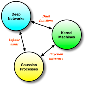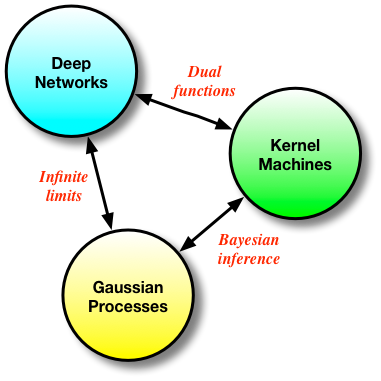
Memory, the ways in which we remember and recall past experiences and data to reason about future events, is a term used frequently in current literature. All models in machine learning consist of a memory that is central to their usage. We have two principal types of memory mechanisms, most often addressed under the types of models they stem from: parametric and non-parametric (but also all the shades of grey in-between). Deep networks represent the archetypical parametric model, in which memory is implemented by distilling the statistical properties of observed data into a set of model parameters or weights. The poster-child for non-parametric models would be kernel machines (and nearest neighbours) that implement their memory mechanism by actually storing all the data explicitly. It is easy to think that these represent fundamentally different ways of reasoning about data, but the reality of how we derive these methods points to far deeper connections and a more fundamental similarity.
Deep networks, kernel methods and Gaussian processes form a continuum of approaches for solving the same problem - in their final form, these approaches might seem very different, but they are fundamentally related, and keeping this in mind can only be useful for future research. This connection is what I explore in this post.
Basis Functions and Neural Networks
All the methods in this post look at regression: learning discriminative or input-output mappings. All such methods extend the humble linear model, where we assume that linear combinations of the input data x, or transformations of it φ(x), explain the target values y. The φ(x) are basis functions that transform the data into a set of more interesting features. Features such as SIFT for images or MFCCs for audio have been popular in the past - in these cases, we still have a linear regression, since the basis functions are fixed. Neural networks give us the ability to use adaptive basis functions, allowing us to learn what the best features are from data instead of designing these by-hand, and allowing for a non-linear regression.
A useful probabilistic formulation separates the regression into systematic and random components: the systematic component is a function f we wish to learn, and the targets are noisy realisations of this function. To connect neural networks to the linear model, I'll explicitly separate the last linear layer of the neural network from the layers that appear before it. Thus for an L-layer deep neural network, I'll denote the first L-1 layers by the mapping φ(x; θ) with parameters θ, and the final layer weights w; the set of all model parameters is q = {θ, w}.
![]()
![]()
Once we have specified our probabilistic model, this implies an objective function for optimising the model parameters given by the negative log joint-probability. We can now apply back-propagation and learn all the parameters, performing MAP estimation in the neural network model. Memory in this model is maintained in the parametric modelling framework; we do not save the data but compactly represent it by the parameters of our model. This formulation has many nice properties: we can encode properties of the data into the function f, such as being a 2D image for which convolutions are sensible, and we can choose to do a stochastic approximation for scalability and perform gradient descent using mini-batches instead of the entire data set. The loss function for the output weights is of particular interest, since it will offers us a way to move from neural networks to other types of regression.
![Rendered by QuickLaTeX.com \[ J(\mathbf{w}) = \frac{1}{2} \sum_{n=1}^{N} (y_n - \mathbf{w}^\top \phi(\mathbf{x}_n; \theta))^2 + \frac{\lambda}{2 }\mathbf{w}^\top\mathbf{w}.\]](https://blog.shakirm.com/wp-content/ql-cache/quicklatex.com-bc5f917fa7167a3c2a28bed1cc92ca3b_l3.png)
Kernel Methods
If you stare a bit longer at this last objective function, especially as formulated by explicitly representing the last linear layer, you'll very quickly be tempted to compute its dual function [cite key="bishop2006pattern"][pp. 293]. We'll do this by first setting the derivative w.r.t. w to zero and solving for it:
![]()
![]()
We've combined all basis functions/features for the observations into the matrix Φ. By taking this optimal solution for the last layer weights and substituting it into the loss function, two things emerge: we obtain the dual loss function that is completely rewritten in terms of a new parameter α, and the computation involves the matrix product or Gram matrix K=ΦΦ'. We can repeat the process and solve the dual loss for the optimal parameter α, and obtain:
![]()
And this is where the kernel machines deviate from neural networks. Since we only need to consider inner products of the features φ(x) (implied by maintaining K), instead of parameterising them using a non-linear mapping given by a deep network, we can use kernel substitution (aka, the kernel trick) and get the same behaviour by choosing an appropriate and rich kernel function k(x, x'). This highlights the deep relationship between deep networks and kernel machines: they are more than simply related, they are duals of each other.
The memory mechanism has now been completely transformed into a non-parametric one - we explicitly represent all the data points (through the matrix K). The advantage of the kernel approach is that is is often easier to encode properties of the functions we wish to represent e.g., functions that are up to p-th order differentiable or periodic functions, but stochastic approximation is now not possible. Predictions for a test point x* can now be written in a few different ways:
![]()
The last equality is a form of solution implied by the Representer theorem and shows that we can instead think of a different formulation of our problem: one that directly penalises the function we are trying to estimate, subject to the constraint that the function lies within a Hilbert space (and providing a direct non-parametric view):
![Rendered by QuickLaTeX.com \[ J(f) =\frac{1}{2} \sum_{n=1}^{N} (y_n - f(\mathbf{x}_n))^2 + \frac{\lambda}{2 }\| f\|^2_{\mathcal{H}}.\]](https://blog.shakirm.com/wp-content/ql-cache/quicklatex.com-fe7a2ce1ed2ca0f9728b8a75b3bfb252_l3.png)
Gaussian Processes
We can go even one step further and obtain not only a MAP estimate of the function f, but also its variance. We must now specify a probability model that yields the same loss function as this last objective function. This is possible since we now know what a suitable prior over functions is, and this probabilistic model corresponds to Gaussian process (GP) regression [cite key="rasmussen2006gaussian"]:
![]()
We can now apply the standard rules for Gaussian conditioning to obtain a mean and variance for any predictions x*. What we obtain is:
![]()
![]()
![]()
Conveniently, we obtain the same solution for the mean whether we use the kernel approach or the Gaussian conditioning approach. We now also have a way to compute the variance of the functions of interest, which is useful for many problems (such as active learning and optimistic exploration). Memory in the GP is also of the non-parametric flavour, since our problem is formulated in the same way as the kernel machines. GPs form another nice bridge between kernel methods and neural networks: we can see GPs as derived by Bayesian reasoning in kernel machines (which are themselves dual functions of neural nets), or we can obtain a GP by taking the number of hidden units in a one layer neural network to infinity [cite key="neal1994priors"].
Summary
Deep neural networks, kernel methods and Gaussian processes are all different ways of solving the same problem - how to learn the best regression functions possible. They are deeply connected: starting from one we can derive any of the other methods, and they expose the many interesting ways in which we can address and combine approaches that are ostensibly in competition. I think such connections are very interesting, and should prove important as we continue to build more powerful and faithful models for regression and classification.
[bibsource file=http://www.shakirm.com/blog-bib/SVDL3.bib]

Two remarks (probably):
1) The objective function at the end of the Neural Network (NN) subsection seems to be a little rare. Up to my knowledge, for a NN, the weight vector is included into the argument of
\phi. That is,

\phi(\sigmain NN literature).2) Up to my knowledge, distinguishing between parametric and non-parametric models depends on if we use a function for modelling the data (e.g. a guassian, a linear, quadratic, etc.), so the parameters of the unique used function make it "parametric". Not so for NNs, where data is modeled by sequences of "knots" (a sequence of subfunctions, which parameters must be learned) http://www.researchgate.net/publication/263597992_Smoothing_Splines_Methods_and_Applications_by_Yuedong_Wang.
3) According to the above, I think the parametric version of a NN es the simple perceptron. For more than one hidden non-linearity, the model a is nonparametric one. The same case for kernel methods, one Gaussian makes a parametric method, while more than one Gaussian makes a non-parametric one (see the representer theorem, which describes a Fourier series, a sequence of knots).
4) Regarding to keeping memory data explicitly stored (the Gram matrix), I think it is not always true. From 2000, probably before, theory about reproducing kernel Hilbert spaces has been developed for computing implicit mappings, in such a way the inner product between the kernel and input data reduces to a evaluation functional. Moreover, kernel methods theory has recently introduced something called "learning with indefinite kernels" (in Krein spaces), where theoretically is explained how kernel machines can work by using sigmoid kernels. That structure is indeed what we can find in neural networks. And what about that machine called "Deep Multiple Kernel Learning"? Thus, probably with some variations (point 1 above), Kernel machines are the same than NNs (but no different things indeed). Which is very probably true is that one model may be the dual of the other one, but only if we talk about of them as different representations of the same thing. Finally, I have not expertise on Gaussian processes, however, in some Functional Analysis course I could see some equivalences between GPs and RKHSs for approximation.
Hey Shakir, enjoyed the discussion of connections between neural nets and kernels.
I wonder, does it ever make sense to use the dual representation in terms of α in some nonlinear optimization that also involves θ?
Have you heard of this work, which uses kernel pca to measure the goodness of a feature space generated by a neural network?
http://www.jmlr.org/papers/volume12/montavon11a/montavon11a.pdf