· Read in 10 minutes · 1800 words · collected posts ·
We all make mistakes, and as is often said, only then can we learn. Our mistakes allow us to gain insight, and the ability to make better judgements and fewer mistakes in future. In their influential paper, the neuroscientists Robert Rescorla and Allan Wagner put this more succinctly, 'organisms only learn when events violate their expectations' [cite key=rescorla1972theory]. And so too of learning in machines. In both brains and machines we learn by trading the currency of violated expectations: mistakes that are represented as prediction errors.
We rely on predictions to aid every part of our decision-making. We make predictions about the position of objects as they fall to catch them, the emotional state of other people to set the tone of our conversations, the future behaviour of economic indicators, and of the potentially adverse effects of new medical treatments. Of the multitude of prediction problems that exist, the prediction of rewards is one of the most fundamental and one that brains are especially good at. This post explores the neuroscience and mathematics of rewards, and the mutual inspirations these fields offer us for the understanding and design of intelligent systems.
Associative Learning in the Brain
A reward, like the affirmation of a parent or the pleasure of eating something sweet, is the positive value we associate to events that are in some way beneficial (for survival or pleasure). We quickly learn to identify states and actions that lead to rewards, and constantly adapt our behaviours to maximise them. This is an ability known as associative learning and leads us, in the framework of Marr's levels of analysis, to an important computational problem: what is the principle of associative learning in brains and machines?
As modern-day neuroscientists, the tools with which we can interrogate the function of the brain are many: psychological experiments, functional magnetic resonance imaging, pharmacological interventions, single-cell neural recordings, fast-scan cyclic voltammetry, optogenetics; all provide us with a rich implementation-level understanding of associative learning at many levels of granularity. A tale of discovery using these tools unfolds.
It begins with the famous psychological experiments of Pavlov and his dogs. Pavlov's experiments identify two types of behavioural phenomena—Pavlovian or classical conditioning, and instrumental conditioning—which in turn identify two distinct reward-prediction problems. Pavlovian conditioning exposes our ability to make predictions of future rewards given a cue (like the sound of a bell that indicates food); instrumental conditioning shows we can predict and select actions that lead to future rewards. When functional MRI is used to obtain blood oxygen-level dependent (BOLD) contrast images of humans performing classical or instrumental conditioning tasks, one particular area of the brain, the striatum, stands out [cite key=o2004dissociable].
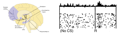
When single-cell recordings of dopaminergic neurons are made from awake monkeys as they reach for a rewarding sip of juice, after seeing a cue (e.g., a light), there is a distinct dopaminergic response [cite key=schultz1992neuronal]. When this reward is first experienced, there is a clear response from dopaminergic neurons, but this fades after a number of trials. The implication is that dopamine is not a representation of reward in the brain. Instead, dopamine was proposed as a means of representing the error made in predicting rewards. A means of causally manipulating multiple neurons is needed to verify such a hypothesis. Optogenetics offers exactly such a tool, and provides a means stimulating precise neural-firing patterns in collections of neurons and observing them by creating a light-activated ion channel. Using optogenetic activation, dopamine neurons were selectively triggered in rats to mimic the effect of positive prediction error, and allowed a causal link between prediction errors, dopamine and learning to be established [cite key=steinberg2013causal].
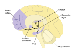
And so goes the reward-prediction error hypothesis: 'the fluctuating delivery of dopamine from the VTA to cortical and subcortical target structures in part delivers information about prediction errors between the expected amount of reward and the actual reward' [cite key = montague1996framework]. There isn't unanimous acceptance of this hypothesis and incentive salience is one alternative [cite key=berridge2007debate]. There is a need for a review that includes the recent evidence that has accumulated, but the existing surveys remain insightful:
- Reinforcement learning in the brain, Y. Niv
- Understanding dopamine and reinforcement learning: The dopamine reward prediction error hypothesis, P. Glimcher.
- Deep and beautiful. The reward prediction error hypothesis of dopamine. M. Colombo.
The reward-prediction error hypothesis is compelling. With support from ever-increasing evidence, we have established the computational problem of associative learning in the brain, an algorithmic solution that predicates learning on prediction errors, and an implementation in brains through the phasic activity of dopaminergic neurons. How can this learning strategy can be used by machines?
Value Learning
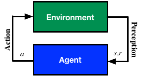
Reinforcement learning—the machine learning of rewards—provides us with the mathematical framework with which we can understand and provide an algorithmic specification of the computational problem of associative learning. As agents in the world, we observe the state of the world s, can take an action a, and observe rewards r, and we do this continually (a perception-action loop). In reinforcement learning the associative learning problem is known as value learning, and involves learning about two types of value function: state value functions and state-action value functions.
![\[\textrm{State value: }V^\pi(s_0) = \sum_t \gamma^t\mathbb{E}_{p_{\pi}(a_t | s_t)p(s_t)}\left[r_t \right]\]](https://blog.shakirm.com/wp-content/ql-cache/quicklatex.com-cb8738c463e03973998883b6ec8125f3_l3.png "Rendered by QuickLaTeX.com")
![\[\textrm{State-action value: }Q^\pi(s_0, a_0) = \sum_{t} \gamma^t\mathbb{E}_{p_{\pi}(a_t | s_t)p(s_t)}\left[r_t \right]\]](https://blog.shakirm.com/wp-content/ql-cache/quicklatex.com-0a3ab70c6d86134dc16736a4e7a2a097_l3.png "Rendered by QuickLaTeX.com")
These equations embody our computational problem:
- We say that the state-value V of a state
![\[s_0\]](https://blog.shakirm.com/wp-content/ql-cache/quicklatex.com-73e131d76bee3b1d76873d8b0e9b709e_l3.png "Rendered by QuickLaTeX.com")
is the discounted sum of all the expected future rewards
![\[r_t\]](https://blog.shakirm.com/wp-content/ql-cache/quicklatex.com-f90d5d867dcf298436b2e2ffde2b5b2c_l3.png "Rendered by QuickLaTeX.com")
that we receive by taking actions
![\[a_t\]](https://blog.shakirm.com/wp-content/ql-cache/quicklatex.com-2977b95097e940d05dbc982f8758d93f_l3.png "Rendered by QuickLaTeX.com")
and reaching state
![\[s_t\]](https://blog.shakirm.com/wp-content/ql-cache/quicklatex.com-b57c7b60fdf1d14f184925dc5c8978f3_l3.png "Rendered by QuickLaTeX.com")
.
- Our actions
are chosen by a policy
![\[\pi\]](https://blog.shakirm.com/wp-content/ql-cache/quicklatex.com-0780e9b463ecc03cc970eb72f6e0b555_l3.png "Rendered by QuickLaTeX.com")
that defines how we behave.
- A discount factor
![\[\gamma\]](https://blog.shakirm.com/wp-content/ql-cache/quicklatex.com-24edd3bc089c270b2a78b63b8ac9f5de_l3.png "Rendered by QuickLaTeX.com")
is introduced, that is between 0 and 1, to include a preference for immediate rewards over distant rewards (and makes the sum finite for bounded rewards).
- The expectation is with respect to the policy
![\[p_\pi(a_t | s_t)\]](https://blog.shakirm.com/wp-content/ql-cache/quicklatex.com-524e6ffe40b164c15da85e62695436ee_l3.png "Rendered by QuickLaTeX.com")
and the marginal state distribution
![\[p(s_t)\]](https://blog.shakirm.com/wp-content/ql-cache/quicklatex.com-52c0f3415b6c82dad73b044d9731ad3b_l3.png "Rendered by QuickLaTeX.com")
(representing all the noisy state transitions and ways in which actions can be selected).
- The state-action value Q is similar, and is the value we associate with state
, when our first action is
![\[a_0\]](https://blog.shakirm.com/wp-content/ql-cache/quicklatex.com-8cec3e3d59b4adc521c5e47413778677_l3.png "Rendered by QuickLaTeX.com")
, but all subsequent actions are taken following the behaviour policy
.
Like in classical conditioning, the state value function
![\[V\]](https://blog.shakirm.com/wp-content/ql-cache/quicklatex.com-77518428ddae5b309efcceea5af87fcc_l3.png "Rendered by QuickLaTeX.com")
allows us to predict future rewards when the right stimuli are present. Like in instrumental conditioning, the state-action value function
![\[Q\]](https://blog.shakirm.com/wp-content/ql-cache/quicklatex.com-002b3d60a76e14deb60893587b7ea3c2_l3.png "Rendered by QuickLaTeX.com")
allows us to select the next action that will allow us to obtain the most reward in future.
In general, there are three ingredients needed for a machine learning solution of a learning problem: a model, a learning objective and an algorithm. There are many types of models we can use to represent value functions: a non-parametric model that maintains a table of values for every state explicitly, a nearest neighbour method or Gaussian process; or a parametric model with parameters
![\[\theta\]](https://blog.shakirm.com/wp-content/ql-cache/quicklatex.com-4c29edd802429cf80b07b851f997cf63_l3.png "Rendered by QuickLaTeX.com")
, such as a deep neural network, a spline model or other basis-function methods.
If we take one step in our environment and move from state
to state
![\[s_{t+1}\]](https://blog.shakirm.com/wp-content/ql-cache/quicklatex.com-da0316ea3f0c56c1dbb8d04d2448fb76_l3.png "Rendered by QuickLaTeX.com")
, the value function should satisfy the following consistency criterion:
![\[V(s_t) = r(s_t,a_t) + \gamma V(s_{t+1})\]](https://blog.shakirm.com/wp-content/ql-cache/quicklatex.com-00ebe3aaeb3d2a7d8ff52098bcf59ff3_l3.png "Rendered by QuickLaTeX.com")
![\[Q(s_t, a_t) = r_t + \gamma \max_a Q(s_{t+1}, a)\]](https://blog.shakirm.com/wp-content/ql-cache/quicklatex.com-a908048192be79d30e4025cc0eb2d4a2_l3.png "Rendered by QuickLaTeX.com")
The self-consistency property of the value function is what we use to obtain our learning objective. The simplest way to do this is to use a measure of discrepancy between the two sides of the equation. For the state value function, we get:
![\[\mathcal{L} = \left(r(s_t,a_t) + \gamma V(s_{t+1}) -V(s_t) \right)^2\]](https://blog.shakirm.com/wp-content/ql-cache/quicklatex.com-236496e02d7382dd754ce5c1e10285c1_l3.png "Rendered by QuickLaTeX.com")
This is known as the squared Bellman residual [cite key=baird1995residual], and importantly, introduces a prediction error that will drive reward-based learning.
We derive a learning algorithm by gradient descent on this objective function. Consider state-value estimation; we obtain two types of descent algorithm, depending on how we treat the term
![\[\nu = r(s_t,a_t) + \gamma V(s_{t+1})\]](https://blog.shakirm.com/wp-content/ql-cache/quicklatex.com-38db1ddc119a53ea8d74029d326dcb67_l3.png "Rendered by QuickLaTeX.com")
, the right-hand side of the Bellman consistency equation.
- Firstly, we can think of
![\[\nu\]](https://blog.shakirm.com/wp-content/ql-cache/quicklatex.com-db2f891c190b5c9e84cef70a0e5d13eb_l3.png "Rendered by QuickLaTeX.com")
as a fixed target for the regression of
to
![\[V(s_t)\]](https://blog.shakirm.com/wp-content/ql-cache/quicklatex.com-50a5839e5302291b5f3915c40ca8c75b_l3.png "Rendered by QuickLaTeX.com")
, in which case
has no parameters.
- In the second case,
is not fixed, and instead forms a residual model that itself has parameters we wish to optimise.
As a result, we obtain two update rules for gradient descent depending on which approach we take, a direct gradient and a residual gradient:
![\[\textrm{Temporal difference: }\delta_t=r(s_t,a_t)+\gamma V(s_{t+1}) -V(s_t)\]](https://blog.shakirm.com/wp-content/ql-cache/quicklatex.com-a2c40df7d6a131f9413452a257c0a875_l3.png "Rendered by QuickLaTeX.com")
![\[\textrm{Direct gradient: }\nabla_\theta \mathcal{L} =\delta_t\nabla_\theta V(s_t)\]](https://blog.shakirm.com/wp-content/ql-cache/quicklatex.com-784d7167d75446bd9c3d6db2ffb5e6ca_l3.png "Rendered by QuickLaTeX.com")
![\[\textrm{Residual gradient: }\nabla_\theta \mathcal{L} =\delta_t\left(\gamma \nabla_\theta V(s_{t+1}) -\nabla_\theta V(s_t) \right)\]](https://blog.shakirm.com/wp-content/ql-cache/quicklatex.com-bb15db60bc51743a43d6e7bb957e23dd_l3.png "Rendered by QuickLaTeX.com")
![\[\textrm{Parameter update: }\theta^{new} = \theta + \eta\nabla_\theta \mathcal{L}\]](https://blog.shakirm.com/wp-content/ql-cache/quicklatex.com-3c671cda07657cbad4eee643582bf4f9_l3.png "Rendered by QuickLaTeX.com")
The term
![\[\delta_t\]](https://blog.shakirm.com/wp-content/ql-cache/quicklatex.com-21bc310a675ed0acf89ee2130e918a5f_l3.png "Rendered by QuickLaTeX.com")
is the temporal difference (TD)—an error in the prediction of rewards at two time points—that quantifies the extent to which our expectations (value predictions) have been violated. Early in learning, our TD errors will be high, and as we learn the TD error fades, shadowing the response of dopamine in the brain (see image).
![Reward prediction errors are high when first encountered, but diminish over time. [Niv, 2009]](https://blog.shakirm.com/wp-content/uploads/2016/02/TDerror-recording.png)
We have derived the famous temporal difference learning algorithm in reinforcement learning [cite key=sutton1998reinforcement], which is the stochastic update rule for parameters of a value function using gradients of the squared Bellman residual. And all this can be repeated for the state-action value function, yielding the Q-learning algorithm. This is a powerful mathematical framework in which to derive a range of more sophisticated reward-based learning systems:
- N-step TD methods
- Instead of forming the consistency equations by rewriting the sum using a reward obtained after 1-step, we can use N-steps of rewards. These are the
![\[TD(\lambda)\]](https://blog.shakirm.com/wp-content/ql-cache/quicklatex.com-54d0605043fa24beb6d40cf866eb073e_l3.png "Rendered by QuickLaTeX.com")
algorithms
.
- Instead of forming the consistency equations by rewriting the sum using a reward obtained after 1-step, we can use N-steps of rewards. These are the
- Fitted and Deep TD methods
- Fitted value function methods make use of rich parametric models and learn these parameters by TD learning. Both Neural fitted Q-learning (NFQ) and Deep Q-Networks (DQN) use deep neural networks to represent the value function, examples of deep reinforcement learning.
- Faster reward learning and alternative algorithms
- We can provide alternative algorithms, and improve performance and reduce estimation biases in many ways. Some of the different approaches we have are delayed Q-learning, phased Q-learning, double Q-learning, reweighted TD update rules such as in emphatic TD, gradient TD (GTD), amongst others.
Final Words
The computational problem of associative learning in the brain is paralleled by value learning in machines. Both brains and machines make long-term predictions about rewards, and use prediction errors to learn about rewards and how to take optimal actions. This correspondence is one of the great instances of the mutual inspiration that neuroscience and machine learning offer each other, more of which we'll explore in other posts in this series.
[bibsource file=http://www.shakirm.com/blog-bib/brainsMachines/temporalDiff.bib]
The explanation of state value (V) and state-action value (Q) based on classical conditioning and instrumental conditioning is really a great "learning" for me.
Amazing article indeed
Thanks for this amazing post.
Translating the math into English in your posts would be terrific !
Cheers !
Amazing and very clear.
Thanks for this clear article.