· Read in 8 minutes ·
Our first encounters with probability are often through a collection of simple games. The games of probability are played with coins, dice, cards, balls and urns, and sticks and strings. Using these games, we built an intuition that allows us to reason and act in ways that account for randomness in the world. But these games are more than just pedagogically powerful—they are also devices we can embed within our statistical algorithms. In this post, we'll explore one of these tools: a stick of length one.
Stick Breaking
I need to probabilistically break a stick that is one unit long. How can I do this? I would need a way to generate a random number between 0 and 1. And once I have this generator, I can generate a random number
![]()
and break the stick at this point. The continuum of points on the unit-stick represents the probability of an event occurring. By breaking the stick in two, I effectively created a probability mass function over two outcomes, with probabilities
![]()
and
![]()
. And I can break these two pieces many more times to obtain a probability mass function over multiple categories, knowing that the sum of all the pieces must be one—the original length of the stick. This gives us an easy way to track how probability can be assigned to a set of discrete outcomes. By controlling how the stick is broken, we can control the types of probability distributions we get. Thus, stick-breaking gives us new ways to think about probability distributions over categories, and hence, of categorical data. Let's splinter sticks in different ways and explore the machine learning of stick-breaking—by developing sampling schemes, likelihood functions and hierarchical models.
Stick-breaking Samplers
The beta distribution is one natural source of random numbers with which to probabilistically break a stick into two pieces. A sample
![]()
lies in the range (0,1), with parameters
![]()
and
![]()
. The essence of stick-breaking is to discover the variable in the range (0,1) hidden within our machine learning problem, and to make it the central character.
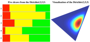
Enter the Dirichlet distribution. The Dirichlet is a distribution over K-dimensional vectors of real numbers in (o,1) where the K-entries sum to one. This makes it a distribution over probability mass functions, and is described by a K-dimensional vector of parameters
![]()
.
![]()
Where is the hidden (0,1)-variable lying in this problem and how can we take advantage of it? The Dirichlet has two very useful properties that addresses these questions.
- The marginal distributions of the Dirichlet are beta distributions.
- Conveniently, the natural tool with which to break a stick is available to us by working with the marginal probabilities. We discover that the Dirichlet distribution is the generalisation of the beta distribution from 2 to K categories.
![Rendered by QuickLaTeX.com \[p(\pi_k) = \mathcal{B}eta\left(\alpha_k, \sum_{i=1}^K \alpha_i - \alpha_k\right)\]](https://blog.shakirm.com/wp-content/ql-cache/quicklatex.com-c63ea5ec025fd5d07790509ec081b3aa_l3.png)
- Conveniently, the natural tool with which to break a stick is available to us by working with the marginal probabilities. We discover that the Dirichlet distribution is the generalisation of the beta distribution from 2 to K categories.
- Conditional distributions are rescaled Dirichlet distributions.
- If we know the probabilities of some of the categories, the probability of the remaining categories is a lower-dimensional Dirichlet distribution. Using
![Rendered by QuickLaTeX.com \[\boldsymbol{\pi}_{\backslash k}\]](https://blog.shakirm.com/wp-content/ql-cache/quicklatex.com-760fc836dcfa4702af5cd1247ec09c85_l3.png)
to represent the vector
![Rendered by QuickLaTeX.com \[\pi\]](https://blog.shakirm.com/wp-content/ql-cache/quicklatex.com-0780e9b463ecc03cc970eb72f6e0b555_l3.png)
excluding the kth entry, and similarly for
![Rendered by QuickLaTeX.com \[\boldsymbol{\alpha}_{\backslash k}\]](https://blog.shakirm.com/wp-content/ql-cache/quicklatex.com-be883e19dfe16d3e8fc970a7a5b7dfb3_l3.png)
, we have:
![Rendered by QuickLaTeX.com \[p(\boldsymbol{\pi}_{\backslash k} | \pi_k) = (1-\pi_k)\mathcal{D}ir(\boldsymbol{\alpha}_{\backslash k})\]](https://blog.shakirm.com/wp-content/ql-cache/quicklatex.com-4c3891ee522a550615069675b52c0dea_l3.png)
- If we know the probabilities of some of the categories, the probability of the remaining categories is a lower-dimensional Dirichlet distribution. Using
Putting these two properties together, we can develop a stick-breaking method for sampling from the Dirichlet distribution [cite key=sethuraman1994constructive]. Consider sampling from a 4-dimensional Dirichlet distribution. We begin with a stick of length one.
- Break the stick in two. We can do this since the marginal distribution for the first category is a Beta distribution.
![Rendered by QuickLaTeX.com \[\sigma_1 \sim \mathcal{B}eta(\alpha_1,\alpha_2 + \alpha_3 +\alpha_4)\]](https://blog.shakirm.com/wp-content/ql-cache/quicklatex.com-4875c0955ab43b0351f68eab5dfb1c30_l3.png)
![Rendered by QuickLaTeX.com \[\pi_1 = \sigma_1\]](https://blog.shakirm.com/wp-content/ql-cache/quicklatex.com-30e8d9ebc1781b0e43d3193214c884fa_l3.png)
- The conditional probability of the remaining categories is a Dirichlet.
![Rendered by QuickLaTeX.com \[p(\pi_2, \pi_3, \pi_4| \pi_1) = (1-\sigma_1)\mathcal{D}ir(\alpha_2, \alpha_3, \alpha_4)\]](https://blog.shakirm.com/wp-content/ql-cache/quicklatex.com-56305e2a07f756ac39513c9c45674bec_l3.png)
- Break the length of the stick that remains into two. The length of the stick that remains is
![Rendered by QuickLaTeX.com \[1-\sigma_1\]](https://blog.shakirm.com/wp-content/ql-cache/quicklatex.com-975ddf13696c464d6fcded7a246fdbfe_l3.png)
, and using the marginal property again:
![Rendered by QuickLaTeX.com \[\sigma_2 = \mathcal{B}eta(\alpha_2 | \alpha_3 +\alpha_4)\]](https://blog.shakirm.com/wp-content/ql-cache/quicklatex.com-c47a96ff66c670aa84769d85f2e3e5de_l3.png)
![Rendered by QuickLaTeX.com \[\pi_2 |\pi_1 \sim(1-\sigma_1)\sigma_2\]](https://blog.shakirm.com/wp-content/ql-cache/quicklatex.com-45d772920bb1a25999aa04d64ef51561_l3.png)
- Repeat steps 2 and 3 for the third category.
![Rendered by QuickLaTeX.com \[\sigma_3 = \mathcal{B}eta(\alpha_3,\alpha_4)\]](https://blog.shakirm.com/wp-content/ql-cache/quicklatex.com-44e1c5829fb0da770a2e065751c377c7_l3.png)
![Rendered by QuickLaTeX.com \[\pi_3 |\pi_1,\pi_2 \sim(1-\sigma_1)(1-\sigma_2)\sigma_3\]](https://blog.shakirm.com/wp-content/ql-cache/quicklatex.com-bdc2497ed0f00c30e56f0aaf4e56ef23_l3.png)
- The remaining length of the stick is the probability of the last category.
![Rendered by QuickLaTeX.com \[p(\pi_4 |\pi_1,\pi_2,\pi_3) =(1-\sigma_1)(1-\sigma_2)(1-\sigma_3)\]](https://blog.shakirm.com/wp-content/ql-cache/quicklatex.com-8bc5b8e489dcb6426b3acaa51f534a50_l3.png)
By repeatedly applying the rules for the marginal and conditional distributions of the Dirichlet, we reduced each of the conditional sampling steps to sampling from a beta distribution—this is the stick-breaking approach for sampling from the Dirichlet distribution.
This is a widely-known alternative sampling process for the Dirichlet distribution.
- Theorem 4.2 of Devroye [cite key=devroye2006nonuniform] is one source of discussion, where it is also contrasted against a more efficient way of generating Dirichlet variables using Gamma random numbers.
- Stick-breaking works because samples from the Dirichlet distribution are neutral vectors: we can remove any category easily and renormalise the distribution using the sum of the entries that remain. This is an inherent property of the Dirichlet distribution and has implications for machine learning that uses it, as we shall see next.
Stick-breaking Likelihoods
Stick-breaking can be used to specify a likelihood function for ordinal (ordered-categorical) data, and by implication, a loss function for learning with ordinal data. In ordinal regression, we are given covariates or features x, and we learn a discriminative mapping to an ordinal variable y using a function
![]()
. Instead of using a beta distribution, we will break the stick at points given by squashing the points on the function through a sigmoid (or probit) function
![]()
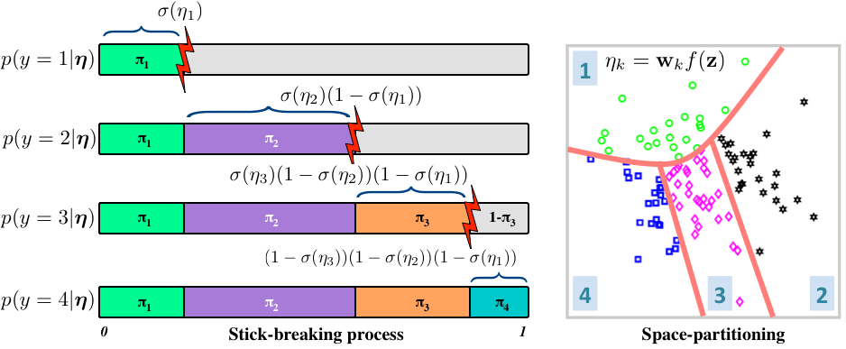
, which is a number in (0,1). If we consider four categories, a stick-breaking likelihood is:
![]()
![]()
![]()
![]()
This is exactly the stick-breaking formulation we used for the Dirichlet distribution, but the parameters are modelled as a function of observed data. The function
![]()
can be any function, e.g., a linear function, deep network or polynomial basis function. The likelihood function carves out the probability space sequentially: each
![]()
defines a decision boundary that separates the kth category from all categories j>k (see figure).
We can compactly write the likelihood as:
![Rendered by QuickLaTeX.com \[ p(y = k |\boldsymbol{\eta}) = \exp\left(\eta_k - \sum_{j < k} \log(1 + \exp(\eta_j))\right) = \frac{\exp(\eta_k)}{\prod_{j < k} 1+\exp(\eta_j)}\]](https://blog.shakirm.com/wp-content/ql-cache/quicklatex.com-5dfd7b6b3939fa0878e691868cea2d78_l3.png)
As a log-likelihood, this gives us one type of loss function for maximum likelihood ordinal regression.
- The stick-breaking likelihood has been used for both regression and density estimation problems as an alternative to the more common cumulative logit for ordinal regression.
- The work by Alan Agresti is one of the most comprehensive references for understanding models of categorical data and their assumptions [cite key=agresti1996introduction].
- This stick-breaking is a generalisation of continuation ratio models, commonly used in item response theory, and allows us to further examine the assumptions that follow as a result of the neutrality property. The specific assumption that we should carefully review is independence of irrelevant alternatives (IIA).
Hierarchical Stick-breaking Models

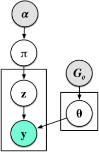
I would like to now consider something far more radical: replacing Dirichlet distributions wherever I find them by stick-breaking representations. Let us experiment with a core model of machine learning—the mixture model. Mixture models with K-components specify the following generative process and graphical model:
-
![Rendered by QuickLaTeX.com \[\boldsymbol{\pi} \sim \mathcal{D}ir\left(\frac{\alpha}{K}, \ldots,\frac{\alpha}{K}\right)\]](https://blog.shakirm.com/wp-content/ql-cache/quicklatex.com-33ddd452d2d7bf5ef2f2809f77e52872_l3.png)
- For c=1, ..., K
-
- For i=1, ..., n
-
In Gaussian mixtures
![]()
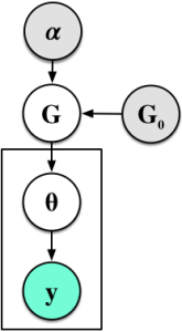
is the distribution of means and variances. When we replace the Dirichlet distribution with a stick-breaking representation we obtain a different, but equivalent, generative process:

- For c=1, ..., K
-
-
![Rendered by QuickLaTeX.com \[G = \sum_{c=1}^K \pi_c \delta_{\phi_c}\]](https://blog.shakirm.com/wp-content/ql-cache/quicklatex.com-18dbc0a8553252683603bab2739c0642_l3.png)
- For i=1, ..., n
-
In the first step, we re-expressed the Dirichlet using the stick-breaking, moving it into the loop over the K categories. We then created a discrete mixture G, where sampling from this chooses one of the mixture parameters with probability
![]()
. The final step is then the same as the original. This view is the random measure view of the mixture model.
We now have an alternative way to express the mixture model that comes with a new set of tools for analysis. We can now be bold enough to ask what happens as the number of clusters
![]()
: obviously, we obtain an infinite mixture model. This is one of the most widely-asked questions in contemporary machine learning and takes us into the domain of Bayesian non-parametric statistics [cite key=hjort2010bayesian].
Today Bayesian non-parametric statistics is the largest consumer of stick-breaking methods and uses them to define diverse classes of highly-flexible hierarchical models.
- The stick-breaking representation provides one way to understand the Dirichlet process (DP).
- We repeatedly broke the part of the stick that remained after every sampling step. What if we continue to break the first part of the stick instead? This is what is used in another type of non-parametric model.
Summary
The analogy of breaking a stick is a powerful tool that helps us to reason about how probability can be assigned to a set of discrete categories. And with this tool, we can develop new sampling methods, loss functions for optimisation, and ways to specify highly-flexible models.
Manipulating probabilities remains the basis of every trick we use in machine learning. Machine learning is built on probability, and the foundations of probability endure as a supply of wondrous tricks that we can use every day.
This series has been a rewarding ramble through different parts of machine learning, and will be the last post in this series—at least for now.
[bibsource file=http://www.shakirm.com/blog-bib/trickOfTheDay/stickbreaking.bib]


![Rendered by QuickLaTeX.com \[\pi_c = \beta_c \prod_{l=1}^{c-1} 1-\beta_l\]](https://blog.shakirm.com/wp-content/ql-cache/quicklatex.com-52848c3350be3f7a56d0c0eccf33f8df_l3.png)
Nice post. BTW, is there a typo p(y=2|η)=(1−σ(η1))σ(η1), should be η2?
Yes, I agree. In the first set of equations in the section Stick-breaking Likelihoods.